Introduction to Vacuum Pressure Measurement

Introduction

The gas pressure within a vessel is defined as the cumulative force exerted on the walls of the vessel by collision of individual gas molecules or atoms with the wall (Figure 1).

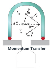
Figure 1. Fundamental source of gas pressure.

Pressure is determined as ^Force/_Area or ^F/_A. The force per unit time exerted on the wall of a container by a single molecule is equal to the momentum transfer between the molecule and the wall and can be expressed as:

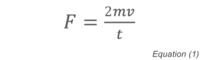
where t is the time between collisions of the molecule with the wall, m is the molecular mass and v its velocity. The pressure can therefore be defined as:

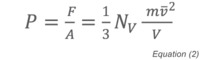
where NV is the total number of molecules in the container, m is the mass of the molecule, v its average velocity, and V the volume of the container. Since the average kinetic energy of a molecule is related to the absolute temperature by:

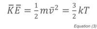
we can substitute and rearrange Equation (2) to become:

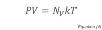
where k is the proportionality constant for the relationship between energy and temperature, known as the Boltzmann constant, and T the absolute temperature. Since the Ideal Gas Constant, R, is just the Boltzmann constant multiplied by Avogadro's Number (N₀, the number of molecules in a mole of substance - 6.022×10²³), Equation (4) is exactly equivalent to the familiar Ideal Gas Law:

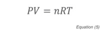
where n is the number of moles of gas and R is the Ideal Gas Constant. The molar volume of a gas is a constant (Avogadro’s Law) with one mole of gas occupying 22.4L at STP (Standard Temperature and Pressure, 1 atmosphere pressure, 0°C). More detailed discussions of the molecular underpinnings of vacuum science and technology can be found in references [1] and [2].

Atmospheric pressure was first measured by the 17th century scientist Evangelista Torricelli. He used an evacuated glass tube that was filled with mercury and then placed upside down in a dish of mercury (this type of measurement device is known as a mercury manometer). Hydrostatic equilibrium requires that the pressure exerted by the column of mercury in the glass tube must equal the pressure exerted by the atmosphere on the mercury in the dish. He found that the force of the atmosphere at sea level on the mercury in the dish would support a column of mercury in the tube that was 760 mm high. This is the reason behind the seemingly odd number of units for atmospheric pressure in this system of measurement - atmospheric pressure was divided into 760 units that are known as "Torr" Vacuum and meteorological measurements in the European and Asian systems usually refer to pressures in "atmospheres" where 1 atmosphere (referred to as 1 bar) is the normal atmospheric pressure at sea level. Vacuum measurements in this system are usually reported in terms of 1/1000th's of an atmosphere (the millibar). The Pascal is the unit used for pressure measurement in the SI system. A Pascal is defined in terms of force per unit area and equals 1 Newton/m².

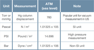
Table 1. Common units of pressure measurement and their value at atmospheric pressure.

Table 1 shows the common units of pressure measurement and their value at atmospheric pressure. A variety of pressure unit conversion calculators can be found online (e.g., https://www.unitconverters.net/pressure-converter.html).

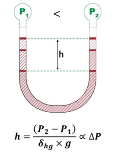
Figure 2. A liquid-filled manometer.

Since Torricelli's time, liquid filled manometers (Figure 2) have remained in use as a fundamental standard for absolute vacuum pressure measurement. Liquid manometers make a direct and absolute measurement of vacuum and pressure, and they are often considered as the fundamental measurement standard to which measurements made by other kinds of pressure measurement devices can be referenced

Modern Pressure Measurement

The most common types of direct pressure measurement use mechanical deformation as the underlying principle for measuring pressure. Since pressure is a measure of force per unit area, differential pressures can deform different kinds of material elements in a reproducible way. The degree of deformation that an element undergoes is proportional to both the material properties of the element and to the pressure exerted on it. Because of this, thin, flexible elements can be used to measure low pressure differentials while thicker, stiffer ones can be similarly used for measuring high pressure differentials. The degree of deflection of these elements can be measured in a variety of ways, including direct mechanical measurement, variation in electrical properties of a device containing the element, and deflection of optical probes.

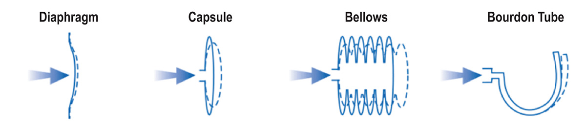
Figure 3. Common mechanical deformation elements used in pressure measurement devices and their mode of deformation with changing pressure.

Figure 3 shows some of the structures that can be employed as deformation elements in a mechanical pressure measurement device. Mechanical deformation gauges include capacitance manometers, Bourdon gauges, resonant diaphragm gauges, bellows gauges, piezoelectric gauges, and others.

Direct pressure measurements at atmospheric and medium vacuum pressures can be determined by measuring the deflection of a thin diaphragm, either metallic or ceramic, in an electromechanical diaphragm gauge (Figure 4). The diaphragm deflection is independent of the gas species present in the gauge and directly proportional to the pressure differential across the diaphragm.

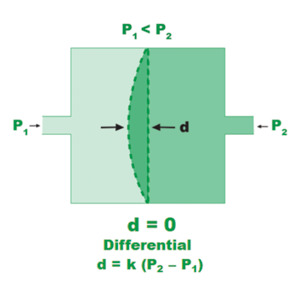
Figure 4. Direct pressure measurement using diaphragm deflection.

Figure 4 shows the relationship between the deflection of the diaphragm and the pressure differential, d, the deflection distance is directly proportional to the pressure difference; the proportionality constant, k, depends on the diaphragm thickness, material, and dimensions. k is determined by calibration against a reference manometer.

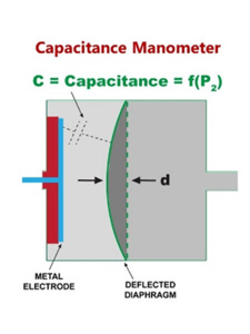
Figure 5. Signal measurement in a capacitance manometer.

Electrical signals proportional to the pressure can be generated by measuring the capacitance between an electrode and the diaphragm (a capacitance manometer, Figure 5). In a capacitance manometer, the diaphragm is deflected toward the lower pressure side as shown in Figure 4. The degree of deflection of the diaphragm in these gauges determines the electrical signal proportional to the pressure difference (P2 – P1) according to the equations shown in Figure 5. In an absolute pressure manometer, one side of the diaphragm (the reference cavity) is a sealed and evacuated cavity in which the pressure is constant and effectively zero. Absolute capacitance manometers are routinely used for process vacuum measurements. The differential pressure across the diaphragm is thus always referenced to vacuum. Differential capacitance manometers do not have a reference cavity – just a tube or passage that can be connected to any pressure or vacuum source. These manometers read the difference in pressure across the diaphragm. Capacitance manometers are vacuum measurement workhorses in the semiconductor industry. Because of their insensitivity to gas composition absolute capacitance manometers are found in almost every semiconductor process tool where they are used to monitor in-process pressures. Differential capacitance manometers find broad application in areas requiring pressure-based switching and control such as chamber load locks. They are routinely used as safety switches and for airflow pressure drop measurements.

The most common commercial electro-mechanical vacuum gauge is exemplified by MKS Instruments' Baratron® capacitance manometer. Baratron capacitance manometers have a high vacuum reference cavity, a welded, corrosion resistant diaphragm sensor, and a counter electrode configured as shown in Figure 6.

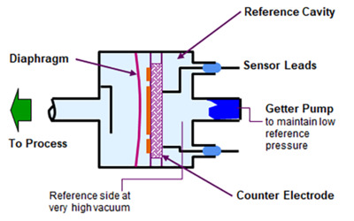
Figure 6. MKS Instruments Baratron® capacitance manometer.

The sealed reference cavity is evacuated to <10^-7 Torr and the vacuum is maintained by a getter pump. Deflection of the diaphragm by high pressure on the measurement side causes an increase in the measured capacitance between the diaphragm and the counter electrode. The change in capacitance unbalances an AC bridge circuit in the instrument, producing a voltage which is rectified and linearized to an analog signal between 0 and 10 VDC that corresponds to 4 decades of dynamic pressure range.

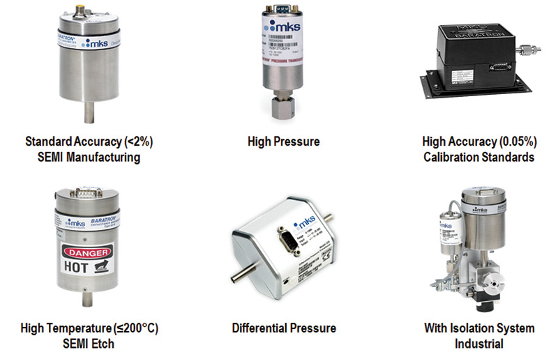
Figure 7. Different types of Baratron® capacitance manometers (10^-5 to 10⁵ Torr).

Figure 7 shows the wide variety of Baratron capacitance manometer configurations that are offered by MKS for different pressure and process environments. These manometers typically measure vacuum over four decades of range. They can be supplied in both heated and unheated versions. Heated versions are most accurate and reliable at >0.1% Full Scale while unheated versions give comparable performance at >0.5% Full Scale. All manometers, regardless of manufacturer, must be periodically zeroed to achieve the best accuracy and repeatability in their measurements. The best zeroing and device accuracy is achieved when the base pressure is <0.01% Full Scale. Baratron capacitance manometers that ranged below 100 mTorr Full Scale should be operated at >1% Full Scale when used in pressure control applications; since pressure control in the lowest decade of the range can be slow and less stable due to noise and A/D resolution limits of the gauge controller (Figure 8).

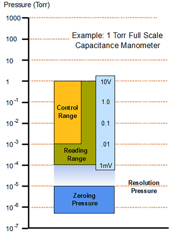
Figure 8. Range and pressure control using Baratron® capacitance manometers.

MKS Instruments supplies both standard and process critical Baratron gauges with high operating temperatures.

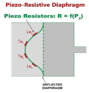
Figure 9. The piezo-resistive diaphragm manometer.

Piezo-resistive pressure manometers are constructed similarly to capacitance manometers but use a piezoresistive element that changes its electrical resistance when strained; these elements are attached to the manometer diaphragm as shown in Figure 9. Piezoresistive elements include film resistors, strain gauges, metal alloys, and polycrystalline semiconductors. When the diaphragm is deflected toward the low-pressure side of the gauge the induced curvature strains the element altering its electrical resistance. This change in resistance is then converted to an electrical output signal using a bridge circuit. These manometers are constructed as shown in Figure 10 which displays the sensing element to the left, the bridge circuitry in the middle, and the physical placement of the sensor in the manometer. The sensors, consisting of a silicon diaphragm, piezo-resistors attached to the diaphragm, sensor leads, and integrated circuitry, are mounted on the reference cavity side of the diaphragm.

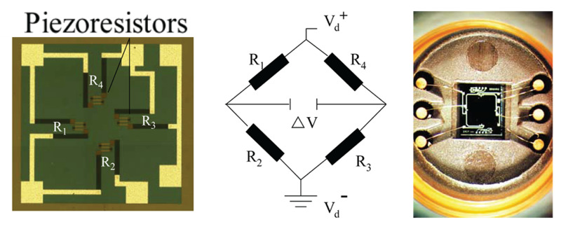
Figure 10. Physical construction of a piezo-resistive manometer showing the bridge circuit.

Piezo-resistive sensors are widely used in both consumer and technological applications. Millions of these are incorporated into tire pressure monitoring devices that can be mounted within the tire on an automobile. MKS Instruments supplies MKS 901P and MKS 902B piezoresistive pressure gauges for technological applications (Figure 11). The MKS 901 sensor is a differential piezoresistive transducer with a range of -760 to 760 Torr that is commonly used in load locks. The MKS 901P can also be configured with a thermal conductivity gauge that extends its range to 5x10^-4 to 1000 Torr for high vacuum load lock applications that makes it well suited for load locks that open to atmosphere and for transfer ports. The MKS 902B is an absolute piezo-resistive transducer with a range from 0.1 to 1000 Torr. It is frequently used in sterile applications such as freeze drying and plasma sterilization. The 902B should not be used for critical measurements below 1 Torr.

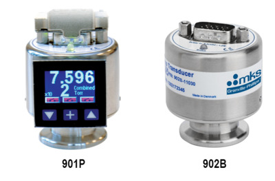
Figure 11. MKS Instruments piezo-resistive 901P and 902B transducers.

At very low pressures (below about 10^-4 Torr), the relative differences between diaphragm deflection measurements at different pressures is no longer sufficiently sensitive for use in a manometer of practical size. Vacuum gauge designs for this pressure regime are therefore based on the measurement of gas density and some species-dependent molecular property such as specific heat. The two main types of these instruments are the thermal conductivity and gas ionization gauges. Thermal conductivity gauges determine gas pressure by measuring the energy transfer from a hot wire to the surrounding gas. The heat is transferred into the gas through molecular collisions with the wire and the frequency of these collisions (and therefore the degree of heat transferred) is dependent on the gas pressure and the molecular weight of the gas molecules. These gauges exhibit simple proportionality between pressure and heat transfer at pressures between 10^-4 and 10 Torr. Thermal conductivity gauges, including thermocouples, thermistors and Pirani gauges are generally relatively inexpensive and reliable.

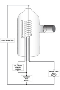
Figure 12. Hot cathode ionization gauge components.

As pressure drops beyond 10^-3 Torr, the variation of thermal conductivity with pressure becomes too small to be useful for pressure measurement. In the high vacuum (below 10^-3 to 10^-9 Torr), ultrahigh vacuum (UHV, 1×10^-9 to 1×10^-12 Torr) and extremely high vacuum (XHV, <1×10^-12 Torr) regimes, pressure measurements most often use gas ionization gauges, configured as either hot cathode gauges (HCIGs) or cold cathode gauges (CCIGs). Both HCIGs and CCIGs determine pressure by measuring the ion flux created by collisions between energetic electrons and residual neutral gas molecules within the gauge. HCIGs employ thermionic emission from a filament as a source of electrons while CCIGs use a circulating space charge to create a free electron plasma. In an HCIG (Figure 12), a filament (the cathode) emits electrons by thermionic emission and a positive electrical potential on the ionization grid accelerates these electrons away from the filament. Electrons oscillate through the grid until they eventually strike either the grid or a molecule of gas. When an electron impacts a gas molecule, a positively charged cation is created that is accelerated toward and collected by a negative electrode known as the collector. The electrical current created in this manner is directly proportional to the number of ions that are created in the gas phase which, in turn, is directly proportional to the gas density and therefore the gas pressure.

Since the physical properties utilized are gas specific, indirect pressure measurement readings are always gas species dependent (i.e. all indirect pressure gauges require gas specific calibration).

Pirani gauges were first developed in the early 1900's. The sensing element is a fine wire of known resistance and known temperature coefficient of resistance (i.e., how its resistance varies with temperature) that is immersed in the gas and electrically heated. The element forms one leg of a balanced Wheatstone bridge. When gas molecules collide with the heated element, they extract heat from it as described above, changing its resistance which unbalances the bridge relative to its reference state. Since the number of collisions and hence the amount of heat transferred to the gas is proportional to the gas pressure, the power required to maintain the bridge in balance is proportional to the pressure. Figure 13 shows a cross-section of a modern MKS Instruments Convectron® Pirani gauge and the power vs. pressure curve for residual nitrogen gas.

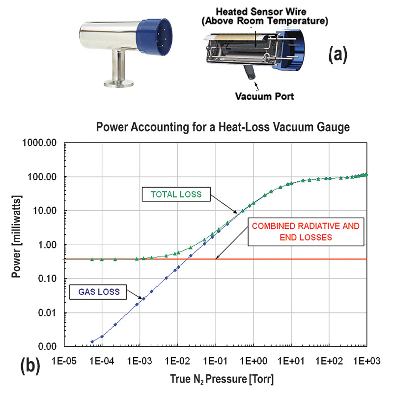
Figure 13. (a) MKS Convectron® Pirani gauge; (b) Power vs. pressure curve for a Pirani gauge in a system with nitrogen residual gas.

The Pirani gauge response to a change in pressure depends on the gas that is present in the system since every gas has a different specific heat capacity. It is also dependent on the molecular mass of the gas and on an accommodation coefficient that accounts for the residence time of the gas molecule in contact with the Pirani element. Users must therefore calibrate a Pirani gauge for the expected residual gas in the system. Figure 14 shows a graphical representation of the response curve (indicated pressure) of a nitrogen-calibrated Pirani gauge for different residual gases that illustrates the importance of proper calibration for a Pirani gauge.

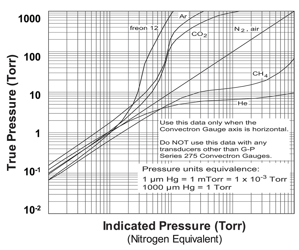
Figure 14. Convectron pressure reading vs. actual pressure for different gases.

In this example, an indicated Argon pressure of 10 Torr represents a true pressure of 1000 Torr. This data makes it clear that improper calibration of a Pirani gauge can lead to severe risk of system over-pressure with consequent safety problems. Additionally, since the Pirani element operates at temperatures between 100 and 150°C, reactive gases that can break down and deposit solid material on the element must be excluded from the gauge. Since heat transfer is significantly reduced below about 10^-4 Torr, Pirani gauge accuracy deteriorates below this pressure. At high pressures (10 Torr and above), the mean free path of gas molecules becomes reduced to a point where nonlinearities enter the pressure-voltage relationship and reduce the gauge's sensitivity. Advanced Pirani gauges are constructed to permit convective forces within the gauge to assist molecular flow. These latter designs enable Pirani gauges to be used with good accuracy up to 760 Torr pressure. Pirani gauges are normally received calibrated for nitrogen and calibration curves are required for use with other gases. Pirani gauges are relatively fast with response to pressure changes occurring in a tenth of a second or less. They are commonly used for pressure indication on vacuum chamber roughing lines, turbopump fore lines, load locks, and for determining chamber pressure for pump and gauge cross-over.

MKS Instruments' 275 Convectron Convection-enhanced Pirani Vacuum Pressure Sensors (Figure 13) and Series 475 gauge controller provide exceptionally stable performance for measurements between 10^-4 Torr to atmospheric pressure. These Pirani transducers employ convection-aided heat loss at higher pressures to extend the maximum accurate pressure measurements of conventional Pirani gauges (typically 10 Torr) to atmospheric pressure. MKS Pirani gauges are available with goldcoated wire (standard) and Pt wire. While gold-coated wire is more accurate, Pt wire is more chemically resistant. MKS Instruments has also leveraged MEMS technology in the design of MicroPirani™ transducers that have faster dynamic response, smaller volumes, and better stability than conventional Pirani gauges. Parylene coating of the MEMS sensor is available for resistance to etching compounds.

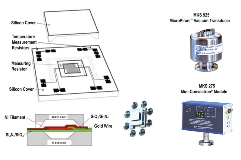
Figure 15. MKS Instruments MicroPirani™ structure and commercial gauges.

Figure 15 shows a schematic of the MicroPirani transducer along with images of two commercial MKS Pirani gauges and systems that employ this technology.

At pressures below 10^-4 Torr, direct pressure measurement methods such as capacitance manometers and Pirani gauges no longer work well, and it becomes necessary to use methods that depend on gas density. Pressure is related to gas density by the expression:

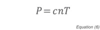
where P is the pressure, c is a constant, n is the number density of the gas, and T is the temperature. As described above, ionization gauges perform this measurement using free electrons that have been produced by either thermionic emission or plasma generation. The ion current that is collected by the negatively biased collector can be related to pressure once the gauge has been calibrated. The basic gauge equation for ionization gauges is:

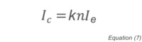
where Ic is the ion current, k is a constant, n is the number density of residual gas molecules and Ie is the ionizing electron current. Substituting for n and rearranging yields an expression for the pressure:

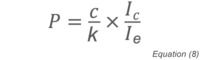
which can be simplified by consolidating constants and defining ionization rate as ^Ic/_Ie:

Where K is a gas-dependent constant determined through calibration and I is the ionization rate proportional to molecular density.

Bayard-Alpert (B-A) Gauges are hot cathode ionization gauges with effective measurement range between 10^-11 and 10^-2 Torr. A hot cathode ionization gauge has three electrodes: the cathode or filament, the collector, and the anode grid. Typically, the collector is at ground potential, the anode at 180V and the filament at 30V. Energetic electrons emitted from the cathode are accelerated towards the anode grid, colliding with and ionizing molecules present in the gas phase. The positive ions that are created in the collisions are accelerated towards the collector located along the axis of the anode grid, producing an ion current that is measured by the gauge electrometer. This gauge configuration produces a strict, linear relationship between collector current and pressure. Thus, the collector is negative relative to the filament and the anode and electrons can only go to the anode. The lower limit for measurement is determined by the X-ray limit. In an HCIG, X-rays are emitted when electrons impact the grid. A small fraction of these X-rays impinges on the ion collector, causing electrons to be ejected by the photoelectric effect. The positive ions created by this ejection of electrons is detected as positive ion current, contributing to the pressure reading. The lower measurement limit in the best conventional HCIGs are about 10^-11 Torr because of this phenomenon. With good operating protocols and proper calibration, the sensor-to-sensor reproducibility of Bayard-Alpert HCIG readings is typically about 2%. Repeatability of readings is 1-2%, limited mainly by uncontrollable random sensitivity variations.

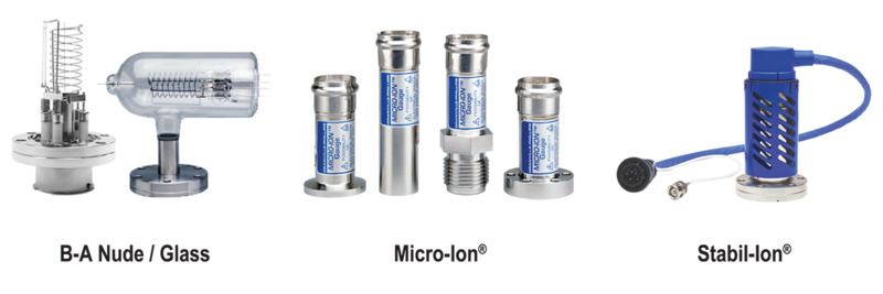
Figure 16. The internal configuration, electron path/ion generation, and physical configuration of a cold cathode ionization gauge.

MKS supplies Bayard-Alpert gauges in several different instrument configurations. Traditional B-A gauges such as the nude or glass-enclosed gauges shown in Figure 16 are a stable, economical solution for the measurement of pressure in high and ultrahigh vacuum regimes. Hot cathode gauges have a repeatability of 1-2%. Glass enclosed gauges typically have gauge-to-gauge reproducibility of ±25% (not tested at factory). The nude gauge configuration has a measurement range between the lower X-ray limit (10^-11 Torr) and 0.001 Torr; the glass-enclosed B-A gauge has a slightly higher lower measurement limit of <1.0x10^-9 Torr. MKS Micro-Ion® Bayard-Alpert gauges are the smallest B-A gauges available, suitable for installation in complex, crowded vacuum systems. They offer a more rugged package than the conventional nude or glass-enclosed gauges that eliminates the risk of glass breakage and ensures long-term stability. Gauge-to-gauge reproducibility of Micro-Ion gauges is ±20% (tested at factory). These gauges have a wider range (5x10^-10 to 5x10^-2 Torr) than the glass-enclosed B-A gauges. MKS Instruments Stabil-Ion® B-A gauge with the Convectron gauge option is a ground-breaking vacuum pressure gauge that offers the widest possible pressure measurement capability (2.0x10^-11 to 999 Torr) and best gauge-to-gauge reproducibility (±6% for the 360 Series and ±4% for the 370 Series) in a rugged package having no potential for glass breakage, glass decomposition, or helium permeation. Stable-Ion gauges are fully electro-statically shielded with a grounded metal gauge tube housing that ensures stable operation in the presence of external electrical interferences. The Stable-Ion gauge is the first ionization gauge with sufficient long-term stability to justify storing calibration data in memory. Each Stabil-Ion gauge is supplied with calibration data based on 15 individually calibrated pressure values. HCGs factory referenced to a Primary Reference Standard (see below) have repeatability of 2-3%.

Cold cathode ionization gauges, CCIGs, also known as Penning gauges, provide effective vacuum pressure measurements between 10^-12 and 10^-2 Torr. This type of ionization gauge uses high (kV) voltage between two electrodes to accelerate random, natural-occurring free electrons (from, e.g. cosmic ray collisions) that collide with residual gas atoms, producing a positive ion and another free electron. The free electrons are captured by the magnetic field, produce an electron plasma. Atoms or molecules within the plasma are ionized and measured as with HCGs. Within the CCIG, the anode is a centrally located rod maintained at high voltage and the cathode is a cylindrical metal cage at ground potential that is concentric with the anode. A ceramic or rare earth magnet surrounds the anode/cathode arrangement (Figure 17a). In operation, crossed electric and magnetic fields control the electron current path, trapping a near-constant circulating electron current in long, cycloidal trajectories within the annulus between the electrodes (Figure 17b). These electrons collide with residual gas molecules creating a positive ion flux at the cathode that is proportional to the number density of residual gas atoms.

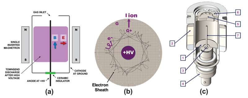
Figure 17. Bayard-Alpert hot cathode ionization gauges available from MKS Instruments.

MKS Instruments supplies cold cathode gauges such as the 971B UniMag™ Cold Cathode vacuum transducer, the 972B DualMag™ Cold Cathode MicroPirani vacuum transducer, and the 974B QuadMag™ Cold CathodeMicroPirani-Piezo vacuum transducer. The 971B UniMag has a measurement range from 1x10^-8 to 5x10^-3 Torr, the DualMag has a range from 1x10^-8 Torr to atmospheric pressure, and the QuadMag gauge has a range from 1x10^-8 Torr to 1500 Torr. As with all ionization gauges, MKS Instruments' HCIG and CCIG gauges must be calibrated for the expected residual gas in the vacuum system. Because of the different operating principle, however, CCIGs require different gas correction factors than those for HCIGs. Repeatability for CCIGs is not normally as consistent as that of HCIGs, with typical values of about ±5% and reproducibility values sensorto-sensor of 30%. For high accuracy operations, CCIGs are normally calibrated against a transfer standard such as a spinning rotor gauge or a high accuracy HCIG. While CCIGs have the advantage of no hot filament that can burn out, they suffer from pressure indication drift over time, discontinuities in pressure indication vs. true pressure, and start-up uncertainties.

Primary Reference Standard Gauges

Spinning Rotor Gauges (SRGs) are a primary reference standard for pressure measurement. Like Pirani gauges, SRGs, also known as molecular drag or viscosity gauges, measure the transfer of energy from a sensor to the surrounding gas to determine the number density of the gas. In the case of the spinning rotor gauge, a small steel ball is magnetically levitated within a non-magnetic tube that is mounted horizontally and connected to the vacuum system. Figure 18 shows a schematic of the SRG.

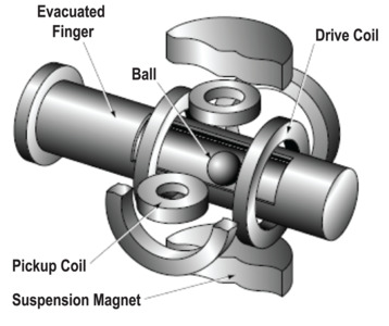
Figure 18. The spinning rotor gauge.

In the measurement procedure, the ball is spun to a few hundred hertz using a rotating magnetic field, then the drive field is turned off and the rate of deceleration of the ball is measured using magnetic sensors. Since the deceleration is caused by the transfer of energy from the ball to gas molecules during collisions, it can be related, using gas kinetic theory, to the number density of the gas and thus to the pressure. SRGs are sensitive to the gas species, and they are often used as a reference gauge for calibrating other gauge types.

Figure 19. The FLOC device optical cavity.

MKS Instruments has collaborated with NIST for the development of a new Pressure Primary Standard based on optical measurements. The Fixed-Length Optical Cavity (FLOC) gauge is a portable device that uses light to measure pressure with higher accuracy and precision than is possible with most commerciallyavailable pressure gauges. It measures subtle differences in the frequency of light passing through two optical cavities, a reference vacuum channel and a channel filled with the gas being measured. A more detailed discussion of the FLOC pressure measurement device can be found at https:// www.nist.gov/news-events/news/2019/02/floc-takesflight-first-portable-prototype-photonic-pressure-sensor.

Conclusion - Vacuum Gauge Selection

Many different types of vacuum gauge are available for applications with different range, accuracy, and materials requirements. The selection of a vacuum gauge for a given vacuum application depends on the expected vacuum environment and the degree of accuracy required for the measurement. For example, a gauge that is expected to measure process pressures during a deposition or etch must, by necessity, be exposed to the process gases. This may impact the measurement accuracy and cause physicochemical problems for the components of the gauge. If a vacuum gauge is needed for the measurement of base pressure in a system in which the chemical nature of residual gases is unknown, gauges in which the measurement has a dependence on the molecular properties of the gas being measured may not be suitable. In a manufacturing environment, it is also important that gauge selection be cost effective. In the case of vacuum gauges, depending on the design and associated ancillary equipment, gauge costs can vary by orders of magnitude. Once the specifications for the vacuum gauge range, accuracy, process compatibility, and cost have been defined, it is important to select the gauge that best matches these specifications.

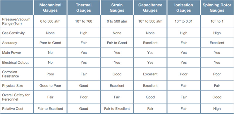
Table 2. Performance and cost comparison for different vacuum gauge types.

Table 2 provides a performance and cost comparison for the different types of vacuum gauges and Figure 20 provides a quick visual guide for the best pressure regimes for using direct and indirect gauges.

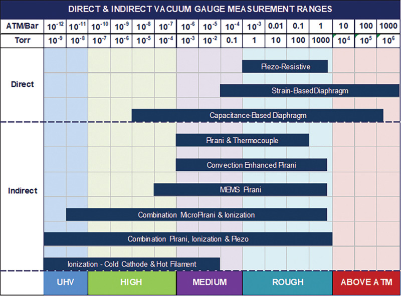
Figure 2. Measurement ranges for direct and indirect vacuum gauges.

[1] A. Roth, Vacuum Technology, Third, Updated and Enlarged ed., Amsterdam: Elsevier Science B. V., 1990.
[2] J. F. O’Hanlon, A User’s Guide to Vacuum Technology, Hoboken, New Jersey: John Wiley & Sons, 2003.